


Results
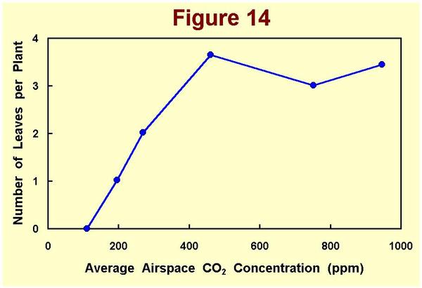 From the large number of measurements we made, we were able to derive several interesting relationships. Figure 14, for example, depicts the mean number of new leaves produced per plant in each CO2 treatment.
 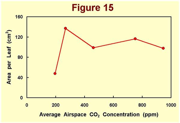 This parameter rises rapidly from a value of zero at 110 ppm to a high of 3.65 at 461 ppm, whereupon the number of leaves per plant rises no further with additional increments of CO2. Leaf area peaked even earlier, at a CO2 concentration of 269 ppm, as shown in Figure 15.
 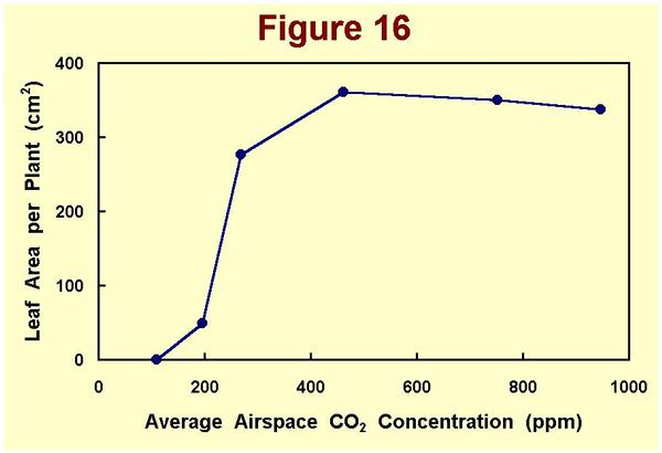 Hence, when corresponding values of these two parameters are multiplied to yield total leaf area per plant, the latter parameter rises extremely rapidly, only to level out above 461 ppm, as depicted in Figure 16.
 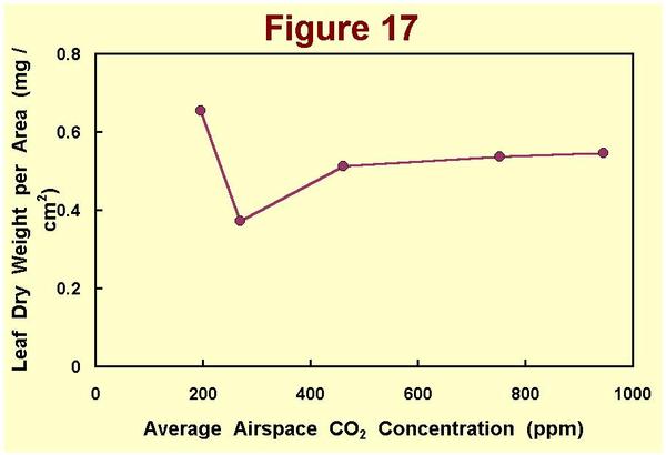 Figure 17 then shows how leaf dry weight per area varied as a function of atmospheric CO2 concentration in our study; and multiplying this parameter by the amount of leaf area per plant produces the leaf dry weight per plant graph of Figure 18.
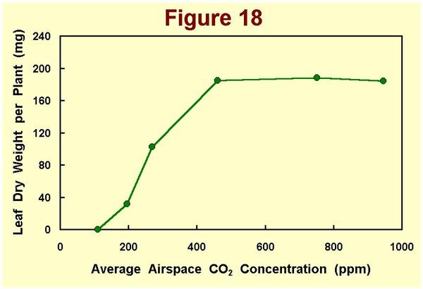 Figure 19 shows how new vine length per plant varied as a function of average airspace CO2 concentration in our experiment; while Figure 20 depicts the relationship we found to prevail between vine dry weight per length and the air's CO2 content.
 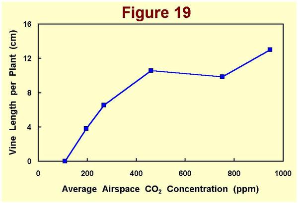 Consequently, multiplying these two parameters produces the vine dry weight per plant relationship of Figure 21, which is comparable in nature to the leaf dry weight per plant relationship of Figure 18.
 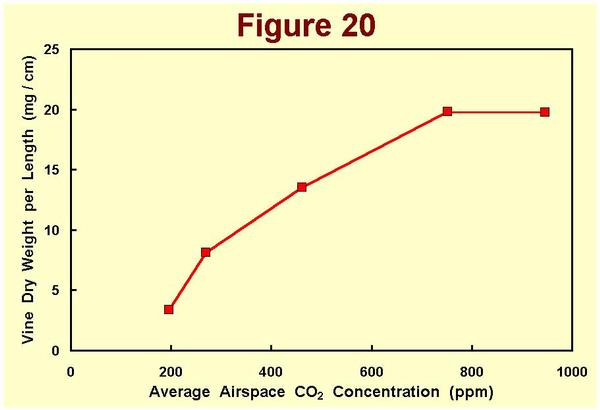 In comparing these two relationships, we see that leaf dry weight per plant only rises with airspace CO2 concentration to a value of 461 ppm, whereas vine dry weight per plant rises all the way out to a CO2 concentration of at least 946 ppm, the highest CO2 concentration achieved in our experiment.
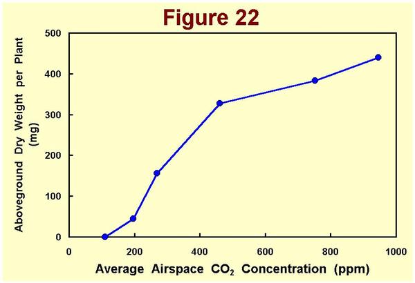
 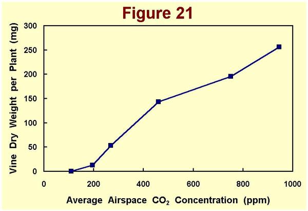 Adding these two relationships then produces the relationship of Figure 22 for total aboveground plant dry weight as a function of atmospheric CO2 concentration.
 Moving to the belowground environment, Figure 23 depicts the numbers of primary, secondary and tertiary roots produced per plant as functions of average airspace CO2 concentration in our experiment; and Figure 24 depicts the mean lengths of each of these types of roots in each of our CO2 treatments.
 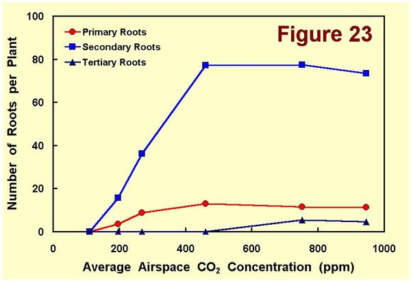 Hence, multiplying corresponding values of these two parameters yields the total root length per plant in each of these root categories as a function of atmospheric CO2 concentration, as shown in Figure 25.
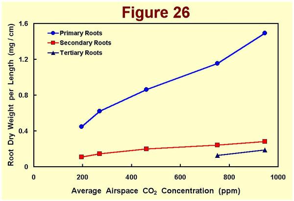
 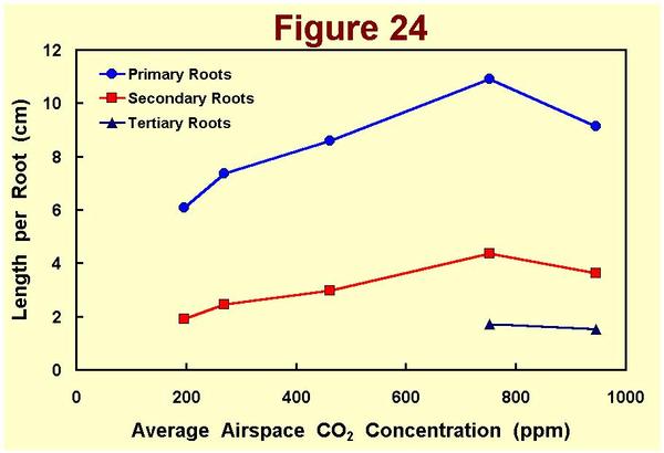 Figure 26 then depicts the relationships we derived between root dry weight per length and atmospheric CO2 concentration for each of the three root categories; and multiplying corresponding values of this parameter and that of Figure 25 produces the root dry weight per plant results of Figure 27.
 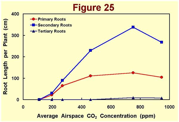 Finally, summing the results of this figure for all three types of roots gives us the total belowground dry weight per plant produced at the several CO2 concentrations of our experiment, as depicted in Figure 28.
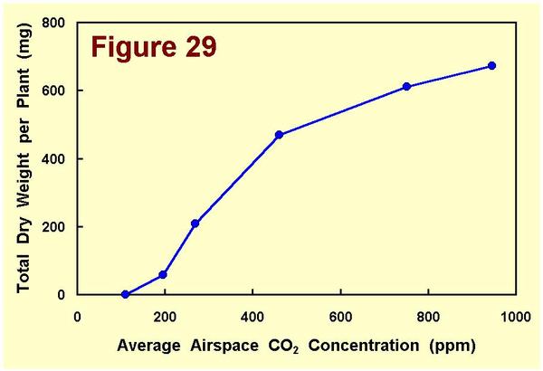
 The final grand concluding graph of our experiment is obtained by adding the aboveground results of Figure 22 and the belowground results of Figure 28.
 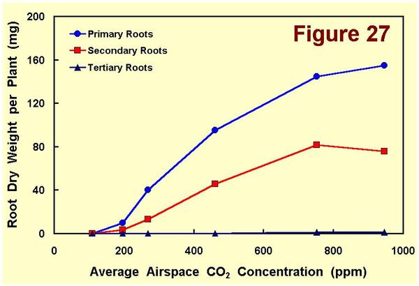 The resulting relationship, depicted in Figure 29, could have been determined much more easily by simply drying the entire intact plants and weighing them.
 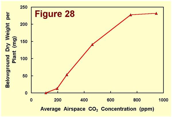 But it wouldn't have been nearly as much fun; and it wouldn't have enabled us to see the many different ways in which the plants responded, part by part, and property by property, to atmospheric CO2 enrichment and depletion.