


Experiment Description
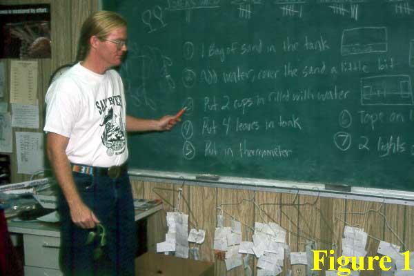 Before the students arrived to start the day, I wrote on our chalkboard the several steps involved in setting up the experiment. Then, when they were settled into their seats and quiet (relatively speaking), I described each of the steps one by one (see Figure 1).
 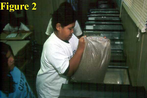 To further help them, I next showed how each step was actually done, so they got to see one of the biospheres being put together from start to finish.
Now it was the students' turn to actually get to work; and to make the potential mayhem more manageable, I divided the class into three groups. 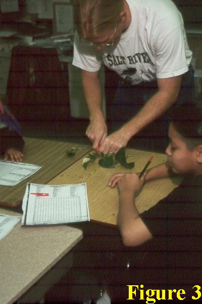 One of them was then allowed to begin setting up the experiment, while the others remained at their desks and worked on a reading assignment. In addition, I assigned each student a partner, so they worked in teams of two.
 The first thing they did was fill each aquarium with a fifty-pound bag of sand, as one of the students is doing in Figure 2. Then they then added just enough water to the sand to totally saturate it when it was smoothed and patted down, after which - if there was not already enough water present - more was added to submerge the top of the sand to a depth of about one centimeter.
 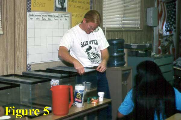 Also at this stage, a glass of water was placed in each end of the aquarium to serve as a source of water for assessing the CO2 content of the biosphere's airspace over the course of the experiment, as described in the Center's CO2 Measurement Technique section.
 Next it was time to introduce the plants into the aquariums. This step was done as described in the Setup Directions for Center Experiment #1, except that for safety's sake, I made all of the cuts on the Pothos vines, but with the students observing closely (see Figure 3).
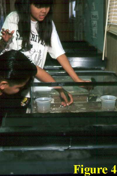
 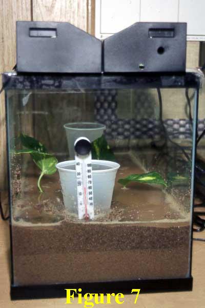 Then each team planted four leaves in each of the aquariums, as two of the students are shown doing in Figure 4.
After putting a thermometer in each tank where it could easily be read (optional), it was time to seal each tank with a thin piece of clear polyethylene, as I am doing in Figure 5, and as is also explained in more detail in the Setup Directions for Center Experiment #1. 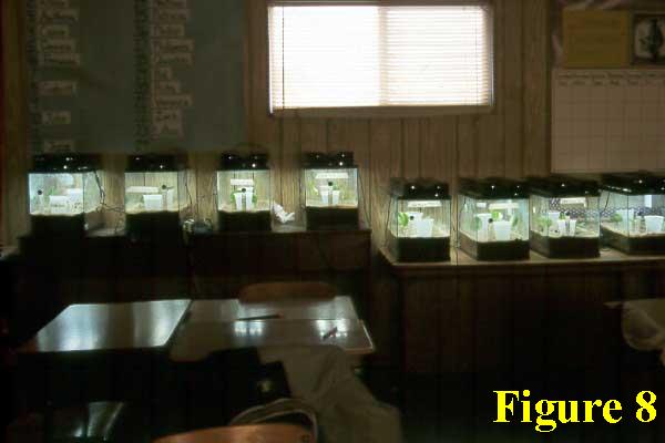 In those directions you can also read how we made a few small holes in the polyethylene tops to establish a range of biospheric airspace CO2 concentrations among our eight experimental units, and how we inserted silicone air tubes into each tank to siphon water out of the glasses located at the ends of each aquarium for making CO2 determinations over the course of the study.
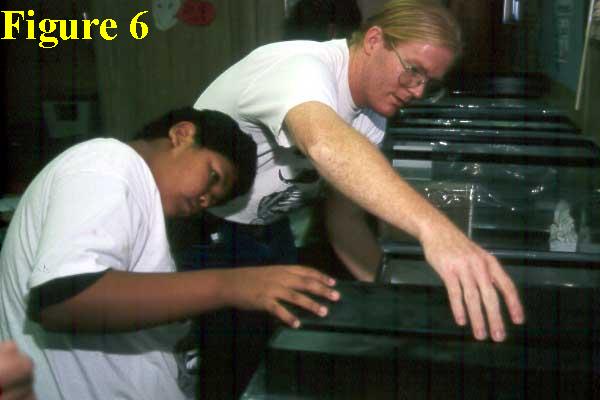
 Last of all, we put two strip-lights containing 15-watt bulbs on the top of each tank, as shown in Figure 6. With this step completed, each tank, when viewed from the end, looked like the one shown in Figure 7; and when the whole class had completed their work, our experiment tables appeared as shown in Figure 8.
 At this point, the experiment had begun; and we made our first CO2 determinations the following day, 16 January, continuing every Monday, Wednesday and Friday until 3 April, after which we harvested the plants on 4 April.
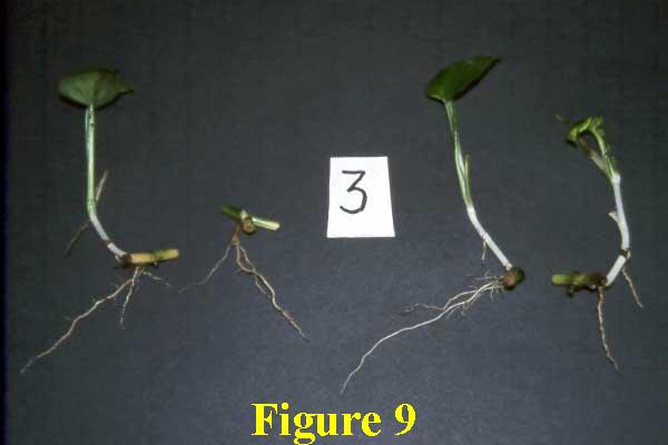
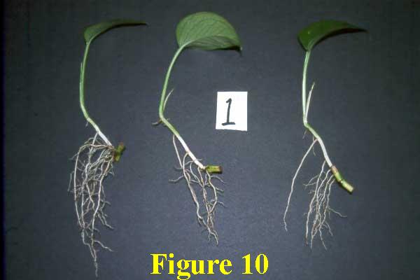
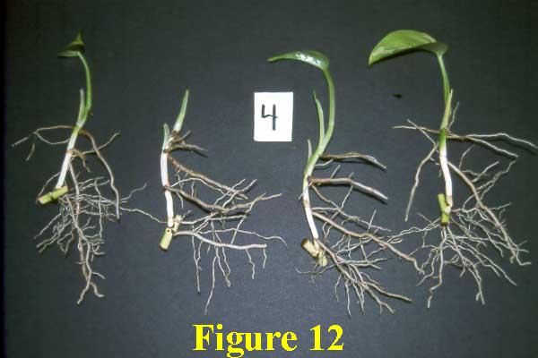
 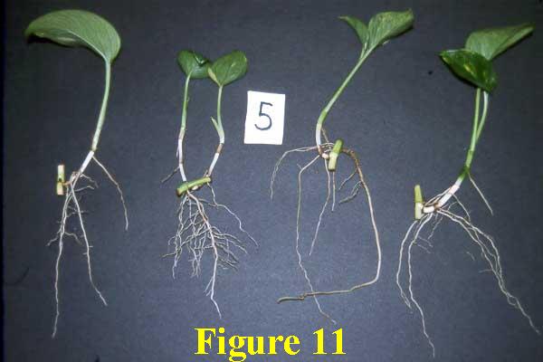 Averaging these data over this eleven-week period, we obtained mean CO2 concentrations ranging from 159 ppm to 638 ppm. Figures 9 - 12 show the plants we harvested from four of these eight experimental units: Tank 3 (159 ppm), Tank 1 (221 ppm), Tank 5 (412 ppm), and Tank 4 (635 ppm).
 Although many types of measurements could have been made on the plants, we merely measured their final fresh and dry weights.